
Often tempting is the search for a receiver with the highest sensitivity. Receiver sensitivity should, however, be balanced against other competing parameters such as dynamic range and selectivity to achieve optimal receiver performance.
Introduction
Communications systems performance emerges from several parameters including sensitivity, dynamic range, selectivity, and power consumption to name a few. These parameters can be in conflict and increasing one parameter may sacrifice performance of another parameter. Further, unique challenges exist in the High Frequency (HF) bands (3-30MHz) due to atmospheric conditions which change dramatically with frequency. Since the selection of a receiver has a tremendous impact on the performance of a communications system, the importance of determining the parameters required for specific operations is paramount. By selecting these parameters wisely, the performance of the receiver can be optimized.
HF Propagation
The HF bands are unique in several ways:
- The absorption of HF signals from various physical properties of materials is generally low.
- HF signals can sometimes reflect, or bounce, off the Earth’s ionosphere, a layer of the Earth’s atmosphere ranging from 50-600 miles above the Earth’s surface.
- Through this ionospheric propagation, also known as skywave propagation, HF signals can travel around the world.
- Skywave propagation is highly variable and is determined by HF frequency, time of day and various environmental conditions.
- HF signals can also travel along the ground using groundwave propagation often beyond line-of-sight.
Due to skywave propagation, the HF bands offer the unique proposition of travelling great distances and providing beyond line-of-site (BLOS) communications capabilities: the ends of a communications circuit can be on opposite sides of the world.
Atmospheric Noise
Manmade and environmental noise will travel the same path as desired signals, raising the noise floor at the receiving end of the BLOS path. These noise sources are prevalent the lower HF bands and significantly raise the noise floor and shown in Figure 1, Atmospheric Noise Floor1. The minimum noise is highlighted by the green line (C & D) while a more worst-case noise level from an urban setting is noted in the line marked E. Note that the Noise Figure (Fa) is significantly higher at 2MHz than at 30MHz. In this case, line D shows the noise figure at 2MHz is approximately 45 – 70dB while at 30MHz it is closer to 20 – 40dB.2
Directional antennas can provide as much as a 10dB improvement of these numbers from elimination of noise in some directions because of the directivity of the antenna. Receiver sensitivity should be set to receive signals just below this noise floor (so as not to add to the noise level), but sensitivity beyond this level provides no benefit since signals will be lost in the atmospheric noise floor. These noise figure numbers will come into play when we look in detail at dynamic range.
1 Further details can be found in ITU-R P.372-8, https://www.itu.int/dms_pubrec/itu-r/rec/p/R-REC-P.372-8-200304-S!!PDF-E.pdf
2 For more background on Noise Figure and the 0dB Noise Figure reference, see https://en.wikipedia.org/wiki/Noise_figure

Dynamic Range
Receivers are called upon to provide clean signals in the presence of other stronger signals. Through digital signal processing (DSP), modern receivers can filter out many adjacent signals that might otherwise cause interference in the reception of the desired signal, but there are limits to this capability. Ultimately, any receiver terminates in a final detector that has a limit on the largest and smallest signal it can represent. For our discussion, we will assume that this final device is an analog to digital converter (ADC). The ADC turns the received analog voltage at any point in time into a numerical representation of that voltage. ADCs typically have a fixed number of output bits and a maximum input voltage. These two parameters set the theoretical wideband dynamic range of the converter. If we take a typical converter with a sampling rate of 250Msps that has a maximum input voltage of 2.5Vpp into a 50-ohm input and a 16- bit output, we can calculate the dynamic range of signals possible:

This result says that in the converter’s full bandwidth, we have a range of signals from +12dBm on the high side and (12 − 96.3) = −84.4dBm on the low side. But there are several factors of importance for an HF receiver that are not taken into account. In a 250Msps converter, we would use a Nyquist filter to capture the first Nyquist zone from 0 − 122.88MHz. The detection bandwidth of our HF receiver is not the width of this Nyquist zone, but is instead something more akin to a 24ksps receiver for a narrowband voice signal. By decimating the converter output down to a rate where we can filter and use just 3kHz of bandwidth we realize the processing gain3 from oversampling4. 4 In this case, that gain is calculated by:
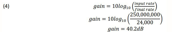
This means that our actual theoretical dynamic range in a 3kHz bandwidth is 96.3dB + 40.2dB = 136.5dB. This is not practically achievable, but it provides a starting point. In order to determine what is possible, we must start with the effective number of bits (ENOB) for the converter5. Ideally a converter would be linear and the data useful over the complete range of bits of output, but noise and distortion limit the effective bits that provide an accurate representation of the analog signal presented to the converter. Let’s assume that the ENOB from our converter is 12.1 bits. Using the formula (2) above tells us that the actual dynamic range afforded by the converter is 20log102(12.1bits); = 72.8dB. This, in turn, gives us our realizable dynamic range in a 3kHz bandwidth as is 72.8dB + 40.2dB = 113.0dB. Without any amplification or attenuation on the input of the converter, our actual dynamic range for a 3kHz signal with this converter would span the range from −101dBm to + 12dBm.
…any given amplifier also has a dynamic range due to its noise figure and overload and if not selected carefully, the amplifier can become the limiting factor in your receiver’s dynamic range.
To provide an idea for what this means in terms of a radio operating on air in an urban setting, the noise floor at 30MHz with typical atmospheric conditions necessitates a receiver with a noise figure around 22dB or better (assuming setting the receiver noise figure 6dB below the atmospheric noise floor). This equates to a noise floor in 3kHz of −125dBm. Our receiver is 24dB worse than it needs to receive a weak signal at 30MHz.
To receive very small signals with the radio, we must provide amplification of the signal before the converter. If we don’t amplify the signal before reaching the converter, the converter cannot represent this small voltage as a number on its output — in short, the converter is not sensitive enough to hear this signal. This is not something that can be done in the digital domain (DSP) after the converter since the information about this weak signal will be lost because the converter cannot sample it. Note also that any given amplifier also has a dynamic range due to its noise figure and overload and if not selected carefully, the amplifier can become the limiting factor in your receiver’s dynamic range. So why not just use an amplifier that would allow us to receive as small a signal as we can imagine in front of the
converter?
3 See https://en.wikipedia.org/wiki/Process_gain
4 See https://www.analog.com/en/technical-articles/analog-tips-decimation-for-adcs.html for more information on decimation.
5 See https://en.wikipedia.org/wiki/Effective_number_of_bits for additional information on ENOB
Sliding Scale
As we noted before, the converter has a fixed signal amplitude range across which it can process signals. This number, the instantaneous dynamic range, is fixed and inherent in the ADC itself. What can be done inside the receiver, is to switch in or out amplification or attenuation of the analog signal before it reaches the ADC. Figure 2, ADC Noise Figure shows our fictional ADC placed “directly on the antenna” with no gain or attenuation. NOISE shown at the bottom of the figure shows where the atmospheric noise level described earlier might be (the actual level will depend on several factors previously discussed including the frequency of interest, propagation conditions, time of day, etc.).
The blue line shows the instantaneous dynamic range of the ADC. As shown, we are sacrificing performance of the receiver near the noise floor and there is a range of signals that we will not be able to hear. Instead, we will hear noise from the receiver in the range noted in red.

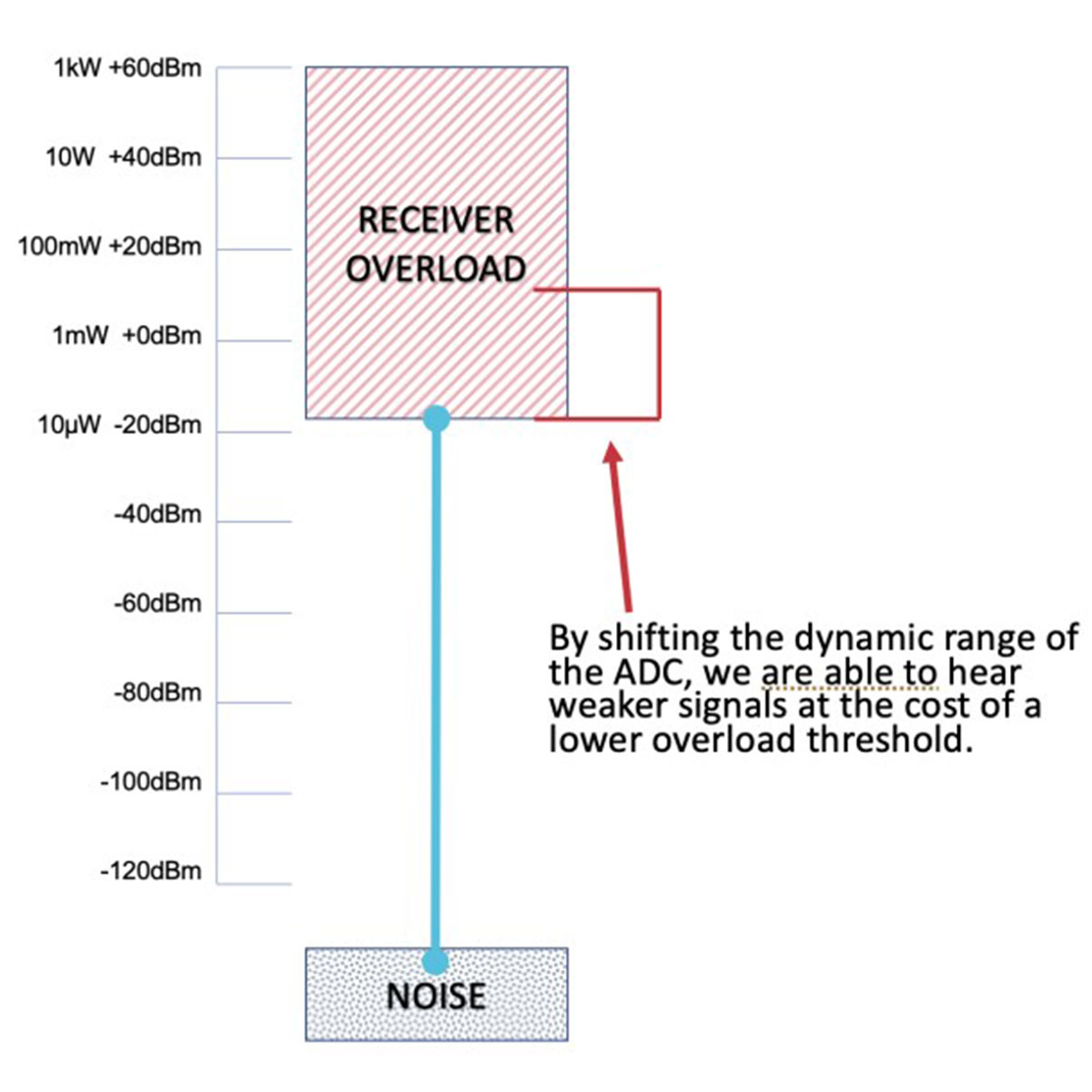
To fix this problem, a preamplification stage can be added to precede the ADC. With a preamplifier, also known as a low-noise amplifier or LNA, we can move the fixed blue line down until it reaches just into the noise floor as shown in Figure 3, Receiver with LNA. The receiver can now hear small signals near the noise floor, but the trade-off made is a shift down of the dynamic range of the converter resulting in reduced receiver overload level. In this fictional case, we have shifted down 30dB, reducing our overload level from +12dBm (16mW) to -18dBm (16µW). Provided that we do not expect signals this large to enter our antenna, the trade-off resulted in a better receiver design that is able to perform across a range of signals.
As a practical matter, receivers often use a couple of different strategies. First, adjustable preamplification where the operator can select, deselect or dial-in a certain amount of amplification can be provided. A second option is to provide automatic gain control (AGC). AGC generally starts with the receiver operating as shown in Figure 3, but if the receiver encounters a large signal and overloads, some or all of the preamplification is switched out, sliding the dynamic range up and preventing future overload.
The key issue with this solution is that an operator listening to a weak signal near the noise floor will encounter what is known as “desensitization” or “desense” where the receiver sensitivity is lowered. This results in a blocking of ability to listen to weak signals because the noise floor rises in the analog circuitry due to the lower sensitivity. In this situation, an operator might comment: “I was desensed by a strong signal in my band of operation.”
An important take-away from this example is that the relative position in the amplitude range of the ADC, in other words where the dynamic range is placed, depends on the type of operation. If the receiver will be used exclusively on strong signals, we might want the receiver to be configured as shown in Figure 2. But if our objective is to listen to weaker signals, Figure 3 is most appropriate. What happens at low frequencies where there is more noise than our 30MHz example?
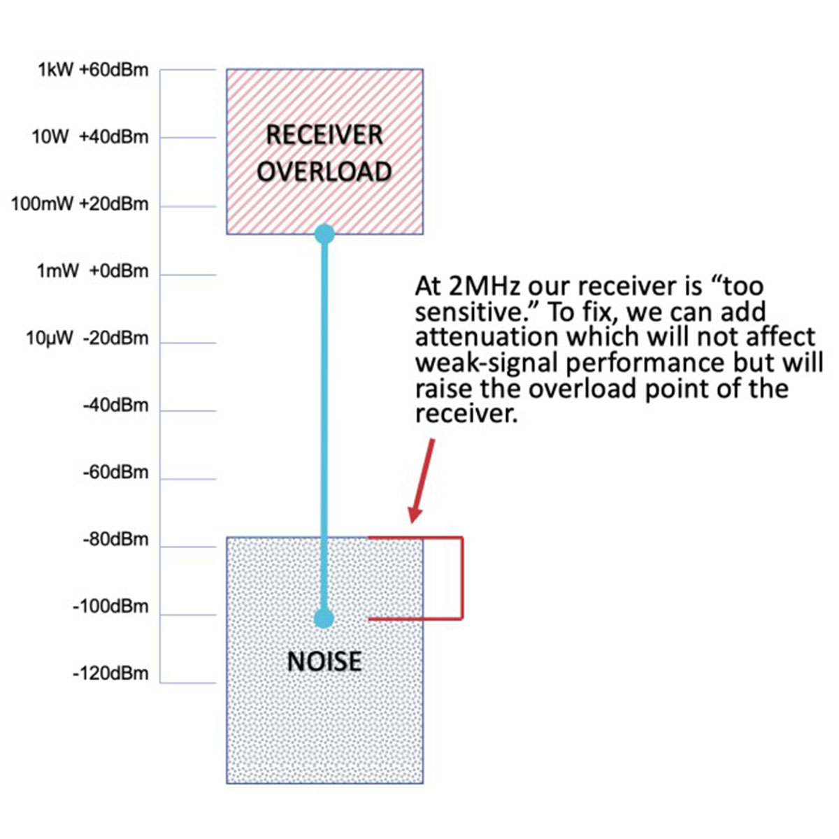
Examining a case where the noise is commensurate with an urban level at 2MHz (65dB noise figure), our starting point with the converter on the antenna yields what we see in Figure 4, “Too sensitive”. In this case, the sensitivity of our radio exceeds the required sensitivity for the atmospheric noise level in the band. As a result, we are wasting dynamic range.
The solution to this problem is to add attenuation in front of the ADC. To the uninitiated, this seems counter-intuitive and counter productive, but we can slide the dynamic range up and add additional overload capability to the receiver for no additional “performance cost.” It is important to mention that all the components in the analog chain must be re-evaluated to ensure that no component is subject to an overload because of this shift. For example, shifting our overload point from +12dBm to +32dBm would require that our attenuator have a input power rating of at least +32dBm (1.6W). These details are handled by the radio designer, but they illustrate some of the tasks required during receiver design.
The receiver dynamic range with the added attenuation can be seen in Figure 5, Attenuation added at low frequencies.

Effects of RMDR
There are other performance parameters in a receiver that can have a deleterious effect on the receiver, even when the receiver is measured to have “excellent sensitivity.” If the receiver can hear very weak signals due to its sensitivity, how could another performance metric affect the receiver and effectively “take away” this sensitivity? Mixing is a necessary function in a modern receiver: it occurs when a frequency of interest is translated, or mixed, to another frequency. This process is undertaken for many reasons in a receiver, including moving the signal from RF frequencies to the audible range that allow us to hear the transmission. Mixing involves the use of a local oscillator (LO) that is used during a mixing or sampling process that translates or samples the RF frequency. Because no oscillators are “perfect,” in this case meaning without noise, additional noise is imparted on all RF signals that are mixed or sampled. This undesirable noise, called phase noise, is added to all signals received as if each of those signals had the noise when they were transmitted.
As a practical matter, phase noise imparted during mixing or sampling is generally not important when imparted to weak signals, but strong received signals can have their occupied bandwidth greatly extended because of this phase noise. When this happens, it is called reciprocal mixing and it can mask out weaker signals that would otherwise be clearly received.
If an LO has phase noise that limits the capabilities of the receiver, reciprocal mixing can overshadow other performance capabilities of the receiver. The phase noise present in the LO is sometimes reported directly and sometimes reported in a performance metric known as Reciprocal Mixing Dynamic Range (RMDR). Whenever the RMDR of a receiver is lower that the dynamic range of the ADC itself, the radio becomes phase noise limited, also known as RMDR-limited. Because receiver testing for sensitivity typically involves testing with a single RF signal (single tone), RMDR limitations are not observed during a sensitivity test when a single, weak signal is present in the receiver. In fact, in the absence of any strong signals, the receiver would perform well as if the RMDR issue was not present. But when a strong signal enters the receiver, the sensitivity is no longer applicable — RMDR would be the limiting factor in receiver performance as it masked out weaker signals.
Summary
Selecting a receiver that has the capability of meeting the sensitivity needs of the operating environment is an important consideration in receiver selection. But the selection of a receiver based solely on the out-of-the-box setting for sensitivity, especially in situations where adjustable gain and attenuation are not available, can sacrifice other key performance metrics such as overload threshold. Other important receive parameters such as RMDR can render an otherwise good dynamic range and sensitivity useless when strong signals are present. Ideally the receiver selected will have overall combined performance characteristics commensurate with the operating and band conditions that exist for the receiver’s mission.